Mini-Project #04: Monte Carlo-Informed Selection of CUNY Retirement Plans
Author
Clinta Puthussery Varghese
INTRODUCTION
In this project, I am tackling a vital personal financial decision using R: selecting a retirement plan as a newly hired faculty member at CUNY. Faculty members have 30 days to choose between two options, and this decision is essentially permanent. Choosing the right plan is no small task—it requires careful analysis of financial trends, demographic assumptions, and personal circumstances. Through this project, I plan to dive into historical financial data and use a bootstrap inference strategy to estimate the probability that one plan outperforms the other. CUNY offers two retirement plans, the traditional defined-benefit Teachers Retirement System (TRS) plan and the newer defined-contribution Optional Retirement Plan (ORP). For this project, I ignore the effect of taxes as both plans offer pre-tax retirement savings, so whichever plan has the greater (nominal, pre-tax) income will also yield the greater (post-tax) take-home amount.
Teachers Retirement System
Employees pay a fixed percentage of their paycheck into the pension fund. For CUNY employees joining after March 31, 2012–which you may assume for this project–the so-called “Tier VI” contribution rates are based on the employee’s annual salary and increase as follows:
$45,000 or less: 3%
$45,001 to $55,000: 3.5%
$55,001 to $75,000: 4.5%
$75,001 to $100,000: 5.75%
$100,001 or more: 6%
The retirement benefit is calculated based on the Final Average Salary of the employee: following 2024 law changes, the FAS is computed based on the final three years salary. (Previously, FAS was computed based on 5 years: since salaries tend to increase monotonically over time, this is a major win for TRS participants.)
If \(N\) is the number of years served, the annual retirement benefit is:
In each case, the benefit is paid out equally over 12 months.
The benefit is increased annually by 50% of the CPI, rounded up to the nearest tenth of a percent: e.g., a CPI of 2.9% gives an inflation adjustment of 1.5%. The benefit is capped below at 1% and above at 3%, so a CPI of 10% leads to a 3% inflation adjustment while a CPI of 0% leads to a 1% inflation adjustment.
The inflation adjustement is effective each September and the CPI used is the aggregate monthly CPI of the previous 12 months; so the September 2024 adjustment depends on the CPI from September 2023 to August 2024.
If N is the number of years served, the annual retirement benefit is: 1.67%FASN if N<=201.75%FASN if N=20 **(35%+2%(N-20))FAS*N if N>=20**
The benefit is increased annually by 50% of the CPI, rounded up to the nearest tenth of a percent: e.g., a CPI of 2.9% gives an inflation adjustment of 1.5%. The benefit is capped below at 1% and above at 3%, so a CPI of 10% leads to a 3% inflation adjustment while a CPI of 0% leads to a 1% inflation adjustment.
The inflation adjustement is effective each September and the CPI used is the aggregate monthly CPI of the previous 12 months; so the September 2024 adjustment depends on the CPI from September 2023 to August 2024.
Optional Retirement Plan
The ORP plan is more similar to a 401(k) plan offered by a private employer. The employee and the employer both make contributions to a retirement account which is then invested in the employee’s choice of mutual funds. Those investments grow “tax-free” until the employee begins to withdraw them upon retirement. If the employee does not use up the funds, they are passed down to that employee’s spouse, children, or other heirs; if the employee uses the funds too quickly and zeros out the account balance, no additional retirement funds are available. Though the employee hopefully still has Social Security retirement benefits and other savings to cover living expenses. This type of plan is called a defined-contribution plan as only the contributions to the retirement account are fixed by contract: the final balance depends on market factors outside of the employee’s control.
At retirement, the employee has access to those funds and can choose to withdraw them at any rate desired. A general rule of thumb is withdrawing 4% of the value per year, e.g., this Schwab discussion; you can assume a constant withdrawal rate in your analysis. Note that unwithdrawn funds continue to experience market returns.
The funds available in a ORP account depend strongly on the investments chosen. For this analysis, you can assume that the ORP participants invest in a Fidelity Freedom Fund with the following asset allocation:[^6]
Age 25 to Age 49:
54% US Equities
36% International Equities
10% Bonds
Age 50 to Age 59:
47% US Equities
32% International Equities
21% Bonds
Age 60 to Age 74:
34% US Equities
23% International Equities
43% Bonds
Age 75 or older:
19% US Equities
13% International Equities
62% Bonds
6% Short-Term Debt
Under the ORP, both the employee and the employer make monthly contributions to the employee’s ORP account. These contributions are calculated as a percentage of the employee’s annual salary. Specifically, the employee contributes at the same rate as the TRS:
$45,000 or less: 3%
$45,001 to $55,000: 3.5%
$55,001 to $75,000: 4.5%
$75,001 to $100,000: 5.75%
$100,001 or more: 6%
The employer contribution is fixed at:
8% for the first seven years of employment at CUNY.
10% for all years thereafter.
DATA SOURCES
For this project, the data are collected from two economic and financial resources: - AlphaVantage: a commercial stock market data provider - FRED: the Federal Reserve Economic Data repository maintained by the Federal Reserve Bank of St. Louis.
convert_fred_datatype=function(fred_data){fred_data=fred_data|>mutate(date=as.Date(date),value=as.numeric(value))|>group_by(date)|>summarise(value =mean(value, na.rm =TRUE), .groups ="drop")return(fred_data)}calculate_return_symbol<-function(alpha_vantage_symbol_data){# Dynamically construct the name for the returns columnreturn_column_name<-paste0(unique(alpha_vantage_symbol_data$symbol), "_returns")}# Define variablesconvert_to_a_table<-function(symbol_data){do.call(rbind, lapply(names(symbol_data$`Monthly Adjusted Time Series`), function(date){# Extract the record for the given daterecord<-symbol_data$`Monthly Adjusted Time Series`[[date]]# Check if all required fields are presentif(!is.null(record$`1. open`)&&!is.null(record$`2. high`)&&!is.null(record$`3. low`)&&!is.null(record$`4. close`)&&!is.null(record$`6. volume`)&&!is.null(record$`7. dividend amount`)){# Create a data frame for non-missing recordsreturn( data=data.frame( date =as.Date(date), # Convert date string to Date open =as.numeric(record$`1. open`), high =as.numeric(record$`2. high`), low =as.numeric(record$`3. low`), close =as.numeric(record$`4. close`), adjusted_close =as.numeric(record$`5. adjusted close`), volume =as.numeric(record$`6. volume`), dividend =as.numeric(record$`7. dividend amount`), stringsAsFactors =FALSE))}else{# Skip records with missing fieldsreturn(NULL)}}))}fetch_alpha_vantage<-function(symbol, function_name="TIME_SERIES_MONTHLY_ADJUSTED"){av_key<-Sys.getenv("AV_KEY")##apikeyurl<-paste0("https://www.alphavantage.co/query?","function=", function_name,"&symbol=", symbol,"&apikey=", av_key)# Make the API requestresponse<-GET(url)if(status_code(response)==200){# Parse and print the JSON datadata<-content(response, as ="parsed")data_table<-data|>convert_to_a_table()data_table=data_table|>mutate(month=floor_date(as.Date(date), "month"))|>group_by(month)|>summarize(adjusted_close =last(adjusted_close))return(data_table)}else{stop("failed to fetch data")}}# Function to fetch data from FREDfetch_fred<-function(series_id){fred_key<-Sys.getenv("FRED_KEY")##apikey for fredreal_time_start="1980-01-01"real_time_end=Sys.Date()frequency="m"url2<-paste0("https://api.stlouisfed.org/fred/series/observations?","series_id=",series_id,"&realtime_start=",real_time_start,"&realtime_end=",real_time_end,"&frequency",frequency,"&api_key=",fred_key,"&file_type=json")response_t=GET(url2)# Check response statusif(status_code(response_t)==200){content<-content(response_t)my_list<-content$observations|>as.list()my_table<-do.call(rbind, lapply(my_list, function(x){data.frame( realtime_start =x$realtime_start, realtime_end =x$realtime_end, date =x$date, value =x$value, stringsAsFactors =FALSE)}))}else{stop("Failed to fetch data from FRED.")}}
DATA ACQUISITION
As the next step, I have collected historical data covering - Rate of Inflation - Rate of Wage Growth - US Equity Market Returns - International Equity Market Returns - Bond Returns - Short Term Debt Returns
FRED Data
Code
# Suppress warnings and messages for better readability of output#| warning: false # Disable warnings#| message: false# Load necessary librarylibrary(lubridate)# For working with dates (e.g., extracting year from a date object)# Disable messages# Fetching and processing inflation data# 1. **Annual Inflation (Percentage)** # Fetches inflation data (consumer prices for the United States) from the FRED API# Converts data types for compatibility and adds a new column for annual CPI percentagesINFLATION_ANNUAL<-fetch_fred(series_id ="FPCPITOTLZGUSA")|>convert_fred_datatype()|>mutate(Annual_CPI_Percentage =value)# 2. **Monthly Inflation Average (Urban Areas)**# Fetches the Consumer Price Index for All Urban Consumers from the FRED API# Renames the `value` column to `US_City_Monthly_Inflation_Average` and `date` to `month` for clarityINFLATION_US_URBAN_AVERAGE<-fetch_fred(series_id ="CPIAUCSL")|>convert_fred_datatype()|>rename(US_City_Monthly_Inflation_Average =value, month =date)
Warning: There was 1 warning in `mutate()`.
ℹ In argument: `value = as.numeric(value)`.
Caused by warning:
! NAs introduced by coercion
Code
# Suppress warnings and messages for better readability of output#| warning: false # Disable warnings#| message: false# 3. **Annual Inflation Average and Percentage Change**# Calculates the annual average of monthly inflation data# Groups data by year, computes the mean for each year, and calculates percentage changes compared to the previous yearannual_inflation_average_percentage<-INFLATION_US_URBAN_AVERAGE|>mutate(year =year(month))|># Extracts year from the month columngroup_by(year)|># Groups data by year for annual summarysummarize( annual_inflation_average =mean(US_City_Monthly_Inflation_Average), # Computes the mean inflation for each year .groups ="drop"# Ungroup data after summarizing)|>mutate( perc_change_annual =(annual_inflation_average-lag(annual_inflation_average))/lag(annual_inflation_average)*100# Computes year-over-year percentage change)# 4. **Monthly Inflation Average (NYC Metro Area)**# Fetches inflation data for the NYC metropolitan area from the FRED API# Converts data types and adds a descriptive column indicating the type of dataINFLATION_NYC<-fetch_fred(series_id ="CUURA101SA0")|>convert_fred_datatype()|>mutate(type ="NYC Monthly Average")
Warning: There was 1 warning in `mutate()`.
ℹ In argument: `value = as.numeric(value)`.
Caused by warning:
! NAs introduced by coercion
Code
# Note:# - `fetch_fred(series_id = "...")`: Retrieves data from the FRED API using the specified series ID.# - `convert_fred_datatype()`: Converts data types to ensure compatibility with further operations.# - `mutate()`: Adds or modifies columns in a data frame.# - `group_by()`: Groups data for aggregation (e.g., summarizing by year).# - `summarize()`: Aggregates data (e.g., computes annual averages).# - `lag()`: Accesses previous row values for calculating percentage changes.
Code
# 5. *Average Hourly Earnings of All Employees, Total Private CES0500000003**# Fetches Average Hourly Earnings of All Employees, Total Private from the FRED API# Converts data types and adds a descriptive column indicating the type of dataWAGE_GROWTH_DATA<-fetch_fred("CES0500000003")|>convert_fred_datatype()|>rename(wage_growth_rate=value,month=date)#6.*Employment Cost Index: Wages and salaries for State and local government workers in Education services (CIU3026100000000I)*WAGE_GROWTH_GOVT_EMPLOYEES<-fetch_fred("CIU3026100000000I")|>convert_fred_datatype()|>rename(wage_growth_rate=value,month=date)
Functions to calculate return:
Code
calculate_return_symbol<-function(alpha_vantage_symbol_data){# Dynamically construct the name for the returns column# Dynamically construct the name for the returns columnreturn_column_name<-paste0(unique(alpha_vantage_symbol_data$symbol), "_returns(%)")ret_vect<-alpha_vantage_symbol_data|>mutate(value=(adjusted_close/lag(adjusted_close)-1)*100,value=round(value,2))|>rename(!!return_column_name:=value)return(ret_vect)}
Functions to calculate long run averages
Code
long_run_monthly_avg<-function(returns_df){return_column_name<-paste0(unique(returns_df$symbol), "_returns(%)")rect_df<-returns_df|>mutate(month_only =format(month, "%m"))|># Extract month (e.g., "01" for January)group_by(month_only)|># Group by monthsummarise( monthly_avg_return =mean(.data[[return_column_name]], na.rm =TRUE)# Calculate the average)return(rect_df)}
ALPHAVANTAGE Data
Code
# Fetching US Equity Market Data Using ETFs# 1. **S&P 500 ETF (SPY)**# Fetches data for SPY ETF from Alpha Vantage, representing the S&P 500 index as a proxy for the US equity market.SPY_ETF<-fetch_alpha_vantage(symbol ="SPY")# Retrieves SPY ETF dataSPY_ETF$symbol<-"SPY"# Adds a new column identifying the symbol for clarity# 2. **Nasdaq-100 ETF (QQQ)**# Fetches data for QQQ ETF from Alpha Vantage, representing the Nasdaq-100 index as another proxy for US equity performance.QQQ_ETF<-fetch_alpha_vantage(symbol ="QQQ")# Retrieves QQQ ETF dataQQQ_ETF$symbol<-"QQQ"# Adds a new column identifying the symbol for clarity# 3. **Dow Jones Industrial Average ETF (DIA)**# Fetches data for DIA ETF from Alpha Vantage, representing the Dow Jones Industrial Average as a proxy for US equity.DIA_ETF<-fetch_alpha_vantage(symbol ="DIA")# Retrieves DIA ETF dataDIA_ETF$symbol<-"DIA"# Adds a new column identifying the symbol for clarity# Calculating Percentage Returns for Each ETF# 4. **Calculate Returns for SPY**# Computes percentage returns for the SPY ETF.usequity1.perc.returns<-calculate_return_symbol(SPY_ETF)# 5. **Calculate Returns for QQQ**# Computes percentage returns for the QQQ ETF.usequity2.perc.returns<-calculate_return_symbol(QQQ_ETF)# 6. **Calculate Returns for DIA**# Computes percentage returns for the DIA ETF.usequity3.perc.returns<-calculate_return_symbol(DIA_ETF)# Combining and Aggregating US Equity Market Returns# 7. **Combine Returns from All ETFs**# Creates a list of percentage returns from SPY, QQQ, and DIA.# Selects only the `month` and the respective return columns for clarity.usequity.all.perc.returns<-list(usequity1.perc.returns|>select(month, `SPY_returns(%)`),usequity2.perc.returns|>select(month, `QQQ_returns(%)`),usequity3.perc.returns|>select(month, `DIA_returns(%)`))|>reduce(full_join, by ="month")|># Merges all three return datasets by `month`arrange(month)|># Ensures data is sorted by `month`drop_na()|># Removes rows with missing datamutate(# Calculates the average return across SPY, QQQ, and DIA to estimate the US equity market return US_equity_market_return =rowMeans(across(c(`SPY_returns(%)`, `QQQ_returns(%)`, `DIA_returns(%)`)), na.rm =TRUE))# Explanation of Functions and Symbols:# - `fetch_alpha_vantage(symbol)`: Fetches ETF data from Alpha Vantage using the specified `symbol`.# - `$symbol`: Adds a new column to label the ETF for later identification.# - `calculate_return_symbol()`: Computes percentage returns for the given ETF data.# - `list()`: Combines selected data frames into a list.# - `select()`: Extracts specific columns (e.g., `month` and returns) for clarity.# - `reduce(full_join, by = "month")`: Merges multiple data frames by the `month` column.# - `arrange(month)`: Ensures the data is chronologically ordered.# - `drop_na()`: Removes rows with missing values to ensure accurate calculations.# - `mutate()`: Creates or modifies columns, e.g., computing the average market return.# - `rowMeans(across(...))`: Computes the average of specified columns row-wise, excluding `NA` values.
Code
# Suppress Warnings and Messages During Execution#| warning: false # Prevents warning messages from being displayed during code execution#| message: false # Suppresses informational messages generated by the functions# Fetching International Equity Market Data Using ETFs# 1. **Vanguard Developed Markets Index Fund ETF (VTMGX)**# Fetches data for the VTMGX ETF, which tracks international developed market equities.VTMGX_INT<-fetch_alpha_vantage(symbol ="VTMGX")|>mutate(symbol ="VTMGX")# Adds a column for identifying the ETF symbol# 2. **Vanguard Emerging Markets Stock Index Fund ETF (VEIEX)**# Fetches data for the VEIEX ETF, which tracks emerging market equities.VEIEX_INT<-fetch_alpha_vantage(symbol ="VEIEX")|>mutate(symbol ="VEIEX")# Adds a column for identifying the ETF symbol# Calculating Percentage Returns for Each International ETF# 3. **Calculate Returns for VTMGX**# Computes percentage returns for the VTMGX ETF.int1.perc.returns<-calculate_return_symbol(VTMGX_INT)# 4. **Calculate Returns for VEIEX**# Computes percentage returns for the VEIEX ETF.int2.perc.returns<-calculate_return_symbol(VEIEX_INT)# Combining and Aggregating International Equity Market Returns# 5. **Combine Returns from VTMGX and VEIEX**# Creates a list containing the percentage returns for both international ETFs.# Selects only the `month` and respective return columns for clarity.int.all.perc.returns<-list(int1.perc.returns|>select(month, `VTMGX_returns(%)`), # Selects monthly returns for VTMGXint2.perc.returns|>select(month, `VEIEX_returns(%)`)# Selects monthly returns for VEIEX)|>reduce(full_join, by ="month")|># Merges the data frames by `month` columnarrange(month)|># Ensures the data is sorted chronologicallydrop_na()|># Removes rows with missing valuesmutate(# Calculates the average return across VTMGX and VEIEX as a proxy for the international equity market return Int_equity_market_return =rowMeans(across(c(`VTMGX_returns(%)`, `VEIEX_returns(%)`)), na.rm =TRUE))# Explanation of Functions and Symbols:# - `fetch_alpha_vantage(symbol)`: Fetches ETF data from Alpha Vantage for the specified `symbol`.# - `mutate(symbol = ...)`: Adds a column to label the ETF for easier identification.# - `calculate_return_symbol()`: Computes percentage returns for the given ETF data.# - `list()`: Combines selected data frames into a list.# - `select()`: Extracts specific columns (e.g., `month` and returns) for clarity.# - `reduce(full_join, by = "month")`: Combines multiple data frames by the `month` column.# - `arrange(month)`: Sorts the data chronologically by `month`.# - `drop_na()`: Excludes rows with missing data for accurate calculations.# - `mutate()`: Creates or modifies columns, e.g., calculating the average international market return.# - `rowMeans(across(...))`: Computes the row-wise average of specified columns, ignoring `NA` values.
Code
# Suppress Warnings and Messages During Execution#| warning: false # Disables warnings#| message: false # Suppresses messages# 1. **Aggregate Bond Index ETF (AGG)**# Fetches data for AGG ETF, a proxy for the aggregate bond market.AGG_BONDS<-fetch_alpha_vantage(symbol ="AGG")|>mutate(symbol ="AGG")# Adds a column to identify the ETF symbol.# 2. **Vanguard Intermediate-Term Corporate Bond Index Fund (VICSX)**# Fetches data for VICSX ETF, representing corporate bond performance.VICSX_BONDS<-fetch_alpha_vantage(symbol ="VICSX")|>mutate(symbol ="VICSX")# Adds a column to identify the ETF symbol.# 3. **Calculating Percentage Returns**# Computes percentage returns for the AGG and VICSX ETFs.bond1.perc.returns<-calculate_return_symbol(AGG_BONDS)bond2.perc.returns<-calculate_return_symbol(VICSX_BONDS)# 4. **Combining and Aggregating Bond Returns**# Merges the percentage returns for AGG and VICSX, calculates average bond market returns.bonds.all.perc.returns<-list(bond1.perc.returns|>select(month, `AGG_returns(%)`), # Selects AGG monthly returnsbond2.perc.returns|>select(month, `VICSX_returns(%)`)# Selects VICSX monthly returns)|>reduce(full_join, by ="month")|># Combines the data frames on `month`arrange(month)|># Sorts by `month`drop_na()|># Removes rows with missing valuesmutate(# Calculates average bond market return Bonds_equity_market_return =rowMeans(across(c(`AGG_returns(%)`, `VICSX_returns(%)`)), na.rm =TRUE))
Code
# Suppress Warnings and Messages During Execution#| warning: false # Disables warnings#| message: false # Suppresses messages# 1. **Vanguard Short-Term Bond Index Fund (VSGDX)**# Fetches data for the VSGDX ETF, representing short-term bond performance.VSGDX_SHORT_TERM<-fetch_alpha_vantage(symbol ="VSGDX")|>mutate(symbol ="VSGDX")# Adds a column to identify the ETF symbol.# 2. **Calculate Short-Term Returns**# Computes percentage returns for the VSGDX ETF.short.term.perc.returns<-calculate_return_symbol(VSGDX_SHORT_TERM)# Optional: Calculate long-run monthly averages if needed# #short.term.long.run.monthly.returns# #long_run_monthly_avg(short.term.perc.returns)
Code
# Suppress Warnings and Messages During Execution#| warning: false # Disables warnings#| message: false # Suppresses messages# Combine all relevant data sources into a single unified dataset.all.data<-list(WAGE_GROWTH_DATA, # Data on wage growthINFLATION_US_URBAN_AVERAGE|>select(month, US_City_Monthly_Inflation_Average), # Inflation datausequity.all.perc.returns|>select(month, US_equity_market_return), # US equity market returnsint.all.perc.returns|>select(month, Int_equity_market_return), # International equity market returnsbonds.all.perc.returns|>select(month, Bonds_equity_market_return), # Bond market returnsshort.term.perc.returns|>select(month, `VSGDX_returns(%)`)# Short-term bond returns)|>reduce(full_join, by ="month")|># Merges datasets on `month`arrange(month)|># Ensures chronological orderdrop_na()# Removes rows with missing values
INITIAL ANALYSIS AND VISUALIZATION OF INPUT DATA
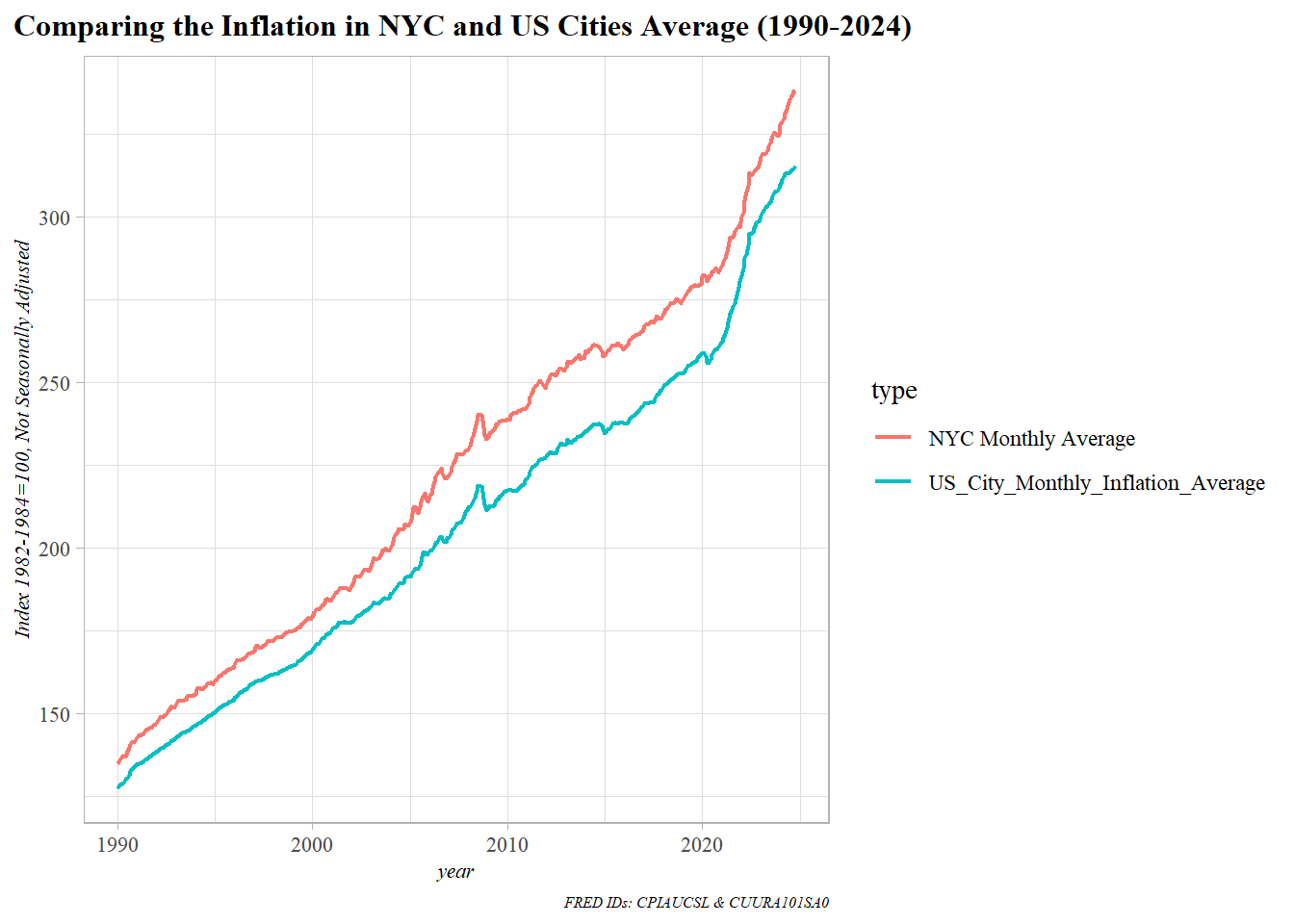
Comparing the Inflation in NYC and US Cities Average (1990-2024)
Code
inflation_us_urban_average=INFLATION_US_URBAN_AVERAGE|>rename(value=US_City_Monthly_Inflation_Average,date=month)|>mutate(type="US_City_Monthly_Inflation_Average")INFLATION_ALL=rbind(inflation_us_urban_average,INFLATION_NYC)ggplot(data =INFLATION_ALL|>filter(year(date)>=1990), aes(x=date, y=value,color=type))+geom_line(linewidth=0.75)+theme_light()+labs(title="Comparing the Inflation in NYC and US Cities Average (1990-2024)", y="Index 1982-1984=100, Not Seasonally Adjusted", x="year", caption ="FRED IDs: CPIAUCSL & CUURA101SA0")+theme(text=element_text(family="serif"), plot.title =element_text(size=12, face="bold"), axis.title =element_text(size=8, face="italic"), plot.caption =element_text(size=6, face="italic"), plot.title.position ="plot")
Montly Adjusted Close Prices of SPY, QQQ, and DIA (US MARKET EQUITY)
Code
US_MARKET_EQUITY=rbind(SPY_ETF,QQQ_ETF,DIA_ETF)gg<-ggplot(US_MARKET_EQUITY, aes(x =month, y =adjusted_close, color =symbol, group =symbol))+geom_line(size =1.2)+labs( title ="Montly Adjusted Close Prices of SPY, QQQ, and DIA (US MARKET EQUITY)", x ="Date", y ="Adjusted Close Price")+theme_bw()ggplotly(gg)
Montly Adjusted Close Prices of VTMGX,VEIEX(INTERNATIONAL_EQUITY)
Code
INTERNATIONAL_MARKET_EQUITY=rbind(VTMGX_INT,VEIEX_INT)gg2<-ggplot(INTERNATIONAL_MARKET_EQUITY, aes(x =month, y =adjusted_close, color =symbol, group =symbol))+geom_line(size =1.2)+labs( title ="Montly Adjusted Close Prices of VTMGX,VEIEX(INTERNATIONAL_EQUITY)", x ="Date", y ="Adjusted Close Price")+theme_bw()ggplotly(gg2)
Montly Adjusted Close Prices of AGG and VICSX(BOND MARKET EQUITY)
Code
BOND_MARKET_EQUITY=rbind(AGG_BONDS,VICSX_BONDS)gg3<-ggplot(BOND_MARKET_EQUITY, aes(x =month, y =adjusted_close, color =symbol, group =symbol))+geom_line(size =1.2)+labs( title ="Montly Adjusted Close Prices of AGG and VICSX(BOND MARKET EQUITY)", x ="Date", y ="Adjusted Close Price")+theme_bw()ggplotly(gg3)
Log10 Monthly Adjusted Close Prices for Bond, International, and US Market Equities
Code
ALL.DATA=rbind(BOND_MARKET_EQUITY|>mutate(type="BONDS"),INTERNATIONAL_MARKET_EQUITY|>mutate(type="INTERNATIONAL"),US_MARKET_EQUITY|>mutate(type="US MARKET"))gg4<-ggplot(ALL.DATA, aes(x =month, y =log10(adjusted_close), color =type, group =symbol))+geom_line(size =1.2)+labs( title ="Log10 Monthly Adjusted Close Prices for Bond, International, and US Market Equities", x ="Date", y ="Log10 Adjusted Close Price")+theme_bw()ggplotly(gg4)
The Bonds Market Equity line exhibits smoother, more stable growth compared to the others, reflecting the generally lower volatility in bond markets.
US Market Equity show greater volatility and fluctuation, characteristic of stock market performance, where prices tend to experience sharper rises and declines.
International Market Equity provides insights into global economic trends, potentially reflecting periods of growth or decline in different countries or regions.
The log10 transformation allows for a more uniform view of percentage changes, making the comparison of relative growth rates more apparent than comparing raw values.
Equal-Weighted U.S. Market Equity Monthly and Annual Returns (SPY, QQQ, DIA)
Warning: There was 1 warning in `mutate()`.
ℹ In argument: `returns = calculate.return(cur_data())`.
ℹ In group 1: `symbol = "DIA"`.
Caused by warning:
! `cur_data()` was deprecated in dplyr 1.1.0.
ℹ Please use `pick()` instead.
Code
US_MARKET_EQUITY_RETURNS<-US_MARKET_EQUITY|>group_by(symbol)|>mutate(returns =calculate.return(cur_data()))|>calculate_monthly_average_return()# Calculate the geometric average annual return (you can choose simple)annual_return<-US_MARKET_EQUITY_RETURNS|>calculate_annual_average_return()# Merge monthly returns with the annual returnsUS_MARKET_EQUITY_RETURNS<-left_join(US_MARKET_EQUITY_RETURNS, annual_return, by=c("year"="year"))ggg<-ggplot(US_MARKET_EQUITY_RETURNS, aes(x =month, y =`average_monthly_return_(%)`))+geom_col(aes(fill =direction), size =1.2)+# Monthly returns as barsgeom_line(aes(x=month,y =`annual_return_(%)` , color ="Annual Return %"), size =1.5)+# Annual return as a linescale_fill_manual(values =c("Increasing"="green", "Decreasing"="red"))+scale_color_manual(values =c("Annual Return %"="blue"))+# Color for the annual return linelabs( title ="Equal-Weighted U.S. Market Equity Monthly and Annual Returns (SPY, QQQ, DIA)", x ="Month", y ="Return (%)", fill ="Monthly Return Direction",)+scale_x_date(date_labels ="%b %Y", date_breaks ="6 months")+# Format x-axis as monthstheme_minimal(base_size =10)+# Larger font size for better readabilitytheme( axis.text.x =element_text(hjust =1), # Rotate x-axis labels for better readability panel.grid.major =element_line(size =0.5, color ="grey"), # Customize gridlines panel.grid.minor =element_blank()# Remove minor gridlines for a cleaner look)
Warning: The `size` argument of `element_line()` is deprecated as of ggplot2 3.4.0.
ℹ Please use the `linewidth` argument instead.
Code
range_from<-as.Date(US_MARKET_EQUITY_RETURNS$year)ggplotly(ggg, dynamicTicks =TRUE)|>layout( xaxis =list(rangeslider =list(borderwidth =1)), # Add range slider to x-axis hovermode ="x", yaxis =list(value =".2f"))# Format ticks as percentage
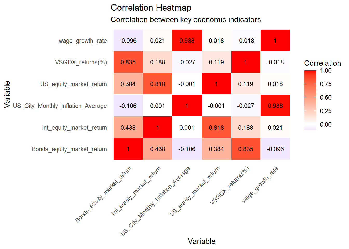
Correlation between key economic indicators
Code
# Calculate the correlation matrixcorrelation_matrix<-all.data%>%select(-month)%>%cor(use ="complete.obs")# Prepare the data for plottingcorrelation_heatmap<-as.data.frame(correlation_matrix)%>%rownames_to_column(var ="variable1")%>%pivot_longer(cols =-variable1, names_to ="variable2", values_to ="correlation")# Create the heatmap with values displayedggplot(correlation_heatmap, aes(x =variable1, y =variable2, fill =correlation))+geom_tile(color ="white")+geom_text(aes(label =round(correlation, 3)), color ="black", size =3)+# Add correlation valuesscale_fill_gradient2(low ="blue", high ="red", mid ="white", midpoint =0)+labs( title ="Correlation Heatmap", subtitle ="Correlation between key economic indicators", x ="Variable", y ="Variable", fill ="Correlation")+theme_minimal()+theme( axis.text.x =element_text(angle =45, hjust =1), panel.grid =element_blank())
wage_growth_rate and US_City_Monthly_Inflation_Average have a high correlation (0.9878), suggesting that as inflation increases, wage growth tends to increase.
US_equity_market_return and wage_growth_rate (0.0184) show almost no relationship. Bonds_equity_market_return and wage_growth_rate (-0.0960) exhibit a slight inverse relationship.
US_equity_market_return and Int_equity_market_return have a strong positive correlation (0.8176), indicating that international and US equity markets move similarly.
Bonds_equity_market_return and VSGDX_returns(%) have a strong positive correlation (0.8354), reflecting alignment between bond and specific equity market returns. -Wage Growth & Inflation: The high correlation (0.9878) between wage growth and inflation suggests that wage adjustments might follow inflation trends.
Equities & Bonds: The mixed correlations (positive and negative) across equity and bond returns reflect diverse market dynamics.
HISTORICAL COMPARISON OF TRS and ORP
I am trying to do a comparison of TRS and ORP with collected historical data. The assumption is the CUNY employee joined the first month of the historical data and retired from CUNY at the end of the final month of data.
Code
#|warning: false##function to calculate TRScalculate_trs<-function(starting_salary, wage_growth_data, inflation_data, years_of_service, retirement_benefit_years){salary<-starting_salarytotal_contributions<-0salaries<-numeric(years_of_service)# Helper function: Calculate biweekly employee contributionsemployee_contribution<-function(salary){emp_rate<-ifelse(salary<=45000, 0.03, ifelse(salary<=55000, 0.035,ifelse(salary<=75000, 0.045,ifelse(salary<=100000, 0.0575, 0.06))))return(salary*emp_rate/26)}# Loop to calculate salary progression and contributionsfor(iin1:years_of_service){annual_increase<-wage_growth_data$annual_ECI_perct[i]/100cpi_rate<-inflation_data$annual_CPI_perct[i]/100salary<-salary*(1+annual_increase+cpi_rate)salaries[i]<-salarybiweekly_contributions<-employee_contribution(salary)total_contributions<-total_contributions+biweekly_contributions*26}# Print Salary Progression for Debuggingprint("\n ::::Year Salary Progression::::::: \n")print(salaries)# Calculate Final Average Salary (FAS)last_3_salaries<-tail(salaries, 3)FAS<-ifelse(length(last_3_salaries)<3, mean(salaries), mean(last_3_salaries))# Helper function: Calculate retirement benefitannual_retirement_benefit<-function(FAS, years_of_service, retirement_benefit_years, inflation_data){if(years_of_service<=20){benefit<-0.0167*FAS*years_of_service}elseif(years_of_service==20){benefit<-0.0175*FAS*years_of_service}else{benefit<-(0.35+0.02*(years_of_service-20))*FAS}return(benefit)}# Calculate the adjusted retirement benefitannual_benefit<-annual_retirement_benefit(FAS, years_of_service, retirement_benefit_years, inflation_data)# Print resultscat("\n Years of Service:", years_of_service, "\n")cat("Final Average Salary (FAS): $", round(FAS, 2), "\n")cat("Total Employee Contributions: $", round(total_contributions, 2), "\n")cat("Annual Retirement Benefit for without Adjustment", retirement_benefit_years, "years: $", annual_benefit, "\n")cat("Monthly Retirement Benefit for without Adjustment", retirement_benefit_years, "years: $", annual_benefit/12, "\n")return(annual_benefit)}
Code
# Define a function to calculate the asset allocation based on agecalculate_allocation<-function(age){# Default asset allocation for all categoriesstocks1_optperc<-0.27/0.55*0.7stocks2_optperc<-0.14/0.55*0.7stocks3_optperc<-0.14/0.55*0.7stocks_optperc<-stocks1_optperc+stocks2_optperc+stocks3_optpercinternational1_optperc<-0.075/0.275*0.15international2_optperc<-0.075/0.275*0.15international3_optperc<-0.125/0.275*0.15international_optperc<-international1_optperc+international2_optperc+international3_optpercbond_optperc<-0shortterm_optperc<-0# Total allocationtotal_optperc<-stocks_optperc+international_optperc+bond_optperc+shortterm_optperc# Determine asset allocation based on ageif(age>=25&age<=49){# Age 25-49: 54% US Equities, 36% International Equities, 10% Bondsstocks_optperc<-0.54international_optperc<-0.36bond_optperc<-0.10}elseif(age>=50&age<=59){# Age 50-59: 47% US Equities, 32% International Equities, 21% Bondsstocks_optperc<-0.47international_optperc<-0.32bond_optperc<-0.21}elseif(age>=60&age<=74){# Age 60-74: 34% US Equities, 23% International Equities, 43% Bondsstocks_optperc<-0.34international_optperc<-0.23bond_optperc<-0.43}elseif(age>=75){# Age 75 and older: 19% US Equities, 13% International Equities, 62% Bonds, 6% Short-Term Debtstocks_optperc<-0.19international_optperc<-0.13bond_optperc<-0.62shortterm_optperc<-0.06}# Calculate total allocation for the specified age rangetotal_optperc<-stocks_optperc+international_optperc+bond_optperc+shortterm_optperc# Return the calculated allocation as a listallocation<-list( stocks =stocks_optperc, international =international_optperc, bonds =bond_optperc, short_term =shortterm_optperc, total =total_optperc)return(allocation)}
Code
#| warning: false#| message: false# Asset returns (annual average return in % for stocks, international, bonds, short term)asset_returns<-c(stocks =all.data$US_equity_market_return, international =all.data$Int_equity_market_return, bonds =all.data$Bonds_equity_market_return, short_term =all.data$`VSGDX_returns(%)`)calculate_orp_with_age<-function(starting_salary, starting_age, wage_growth_data, inflation_data, years_of_service, asset_returns){salary<-starting_salarytotal_balance<-0current_age<-starting_age# Check for NA values in wage_growth_data and inflation_dataif(any(is.na(wage_growth_data$annual_ECI_perct))){warning("Wage growth data contains NA values. Please check the data.")}if(any(is.na(inflation_data$annual_CPI_perct))){warning("Inflation data contains NA values. Please check the data.")}# Helper function: Calculate employee contribution rateemployee_contribution_rate<-function(salary){if(is.na(salary)){stop("Salary is NA. Please provide a valid salary.")# Stop execution if salary is NA}if(salary<=45000)return(0.03)elseif(salary<=55000)return(0.035)elseif(salary<=75000)return(0.045)elseif(salary<=100000)return(0.0575)elsereturn(0.06)}# Loop through each year of servicefor(iin1:years_of_service){# Ensure wage_growth_data and inflation_data have valid entriesif(i<=nrow(wage_growth_data)){annual_increase<-wage_growth_data$annual_ECI_perct[i]/100}else{annual_increase<-0}if(i<=nrow(inflation_data)){cpi_rate<-inflation_data$annual_CPI_perct[i]/100}else{cpi_rate<-0}# Update salary considering wage growth and inflationsalary<-salary*(1+annual_increase+cpi_rate)# Validate salary before calculating contributionsif(is.na(salary)||salary<=0){stop("Salary is invalid or less than zero after adjustments. Please check the data.")}emp_rate<-employee_contribution_rate(salary)emp_contrib<-emp_rate*salaryemp_monthly<-emp_contrib/12employer_rate<-ifelse(i<=7, 0.08, 0.10)employer_contrib<-employer_rate*salaryemployer_monthly<-employer_contrib/12monthly_contrib<-emp_monthly+employer_monthly# Get the asset allocation based on the current ageallocation<-calculate_allocation(current_age)# Annual growth of the portfolio based on asset returns and allocationannual_growth_rate<-sum(c(allocation$stocks/100, allocation$international/100, allocation$bonds/100, allocation$short_term/100)*asset_returns)/100total_balance<-(total_balance+monthly_contrib*12)*(1+annual_growth_rate)current_age<-current_age+1# Increment age by 1 year}# Calculate 4% withdrawal strategyannual_payout<-total_balance*0.04monthly_payout<-annual_payout/12# Return total balance at retirement and the payoutsresult<-list( total_balance =total_balance, annual_payout =annual_payout, monthly_payout =monthly_payout)return(result)}
Testing the functions for the hypothetical employee
Code
# Example usage:starting_salary<-50000# Compute the annual ECI and CPIwage_growth_data<-WAGE_GROWTH_GOVT_EMPLOYEES|>select(month, wage_growth_rate)|>mutate(year =year(month))|>group_by(year)|>summarize(annual_ECI =mean(wage_growth_rate, na.rm =TRUE))|>mutate(annual_ECI_perct =((annual_ECI-lag(annual_ECI))/lag(annual_ECI))*100)|>filter(year>=year(min(all.data$month)))|>na.omit()inflation_data<-INFLATION_US_URBAN_AVERAGE|>select(month, US_City_Monthly_Inflation_Average)|>mutate(year =year(month))|>group_by(year)|>summarize(annual_CPI =mean(US_City_Monthly_Inflation_Average, na.rm =TRUE))|>mutate(annual_CPI_perct =((annual_CPI-lag(annual_CPI))/lag(annual_CPI))*100)|>filter(year>=year(min(all.data$month)))|>na.omit()# Calculate years of serviceyears_of_service<-as.integer(difftime(max(all.data$month), min(all.data$month), units ="days")/365.25)retirement_benefit_years<-15#when I joined the data, it seems like the starting year is 2010. hence 15 years expecting the employee joined around 2010 and retiring 2025# Test the functionannual_benefit=calculate_trs(starting_salary, wage_growth_data, inflation_data, years_of_service, retirement_benefit_years)
[1] "\n ::::Year Salary Progression::::::: \n"
 [1] 51472.86 53592.45 55234.68 56583.94 58251.44 59399.69 61231.94 63747.39
 [9] 66594.78 69547.60 71899.83 76593.04 85258.51 92544.89

 Years of Service: 14
Final Average Salary (FAS): $ 84798.82
Total Employee Contributions: $ 43617.19
Annual Retirement Benefit for without Adjustment 15 years: $ 19825.96
Monthly Retirement Benefit for without Adjustment 15 years: $ 1652.164
Code
# Adjust benefit for inflation during retirementfor(yearin1:retirement_benefit_years){if(year>nrow(inflation_data))breakcpi_adjustment<-inflation_data$annual_CPI_perct[year]/100annual_benefit<-annual_benefit*(1+cpi_adjustment)cat("Inflation Adjusted Annual Benefits for Year",year,":","$",annual_benefit,"\t Monthly Benefits:","$",annual_benefit/12,"\n")}
Inflation Adjusted Annual Benefits for Year 1 : $ 20151.4    Monthly Benefits: $ 1679.283
Inflation Adjusted Annual Benefits for Year 2 : $ 20784.39   Monthly Benefits: $ 1732.033
Inflation Adjusted Annual Benefits for Year 3 : $ 21215.68   Monthly Benefits: $ 1767.974
Inflation Adjusted Annual Benefits for Year 4 : $ 21526.12   Monthly Benefits: $ 1793.843
Inflation Adjusted Annual Benefits for Year 5 : $ 21872.79   Monthly Benefits: $ 1822.732
Inflation Adjusted Annual Benefits for Year 6 : $ 21899.15   Monthly Benefits: $ 1824.929
Inflation Adjusted Annual Benefits for Year 7 : $ 22176.74   Monthly Benefits: $ 1848.061
Inflation Adjusted Annual Benefits for Year 8 : $ 22651.06   Monthly Benefits: $ 1887.588
Inflation Adjusted Annual Benefits for Year 9 : $ 23202.59   Monthly Benefits: $ 1933.549
Inflation Adjusted Annual Benefits for Year 10 : $ 23622.97      Monthly Benefits: $ 1968.581
Inflation Adjusted Annual Benefits for Year 11 : $ 23918.17      Monthly Benefits: $ 1993.18
Inflation Adjusted Annual Benefits for Year 12 : $ 25038.48      Monthly Benefits: $ 2086.54
Inflation Adjusted Annual Benefits for Year 13 : $ 27038.79      Monthly Benefits: $ 2253.232
Inflation Adjusted Annual Benefits for Year 14 : $ 28155.7   Monthly Benefits: $ 2346.308
Inflation Adjusted Annual Benefits for Year 15 : $ 28924.38      Monthly Benefits: $ 2410.365
Code
#Test the function with valid datastarting_salary<-50000starting_age<-50years_of_service<-15#annual.return=all.data|>select(US_equity_market_return,month)|>group_by(year(month))|>result<-calculate_orp_with_age(starting_salary, starting_age, wage_growth_data, inflation_data, years_of_service, asset_returns)# Print resultscat("Total fund at retirement: $", round(result$total_balance, 2), "\n")
Stability and Predictability: TRS is a better option for individuals seeking guaranteed income with less risk and no need for active fund management.
Higher Potential Income: ORP is advantageous for individuals willing to manage their investments, providing higher payouts and financial flexibility, albeit with market-dependent risks.
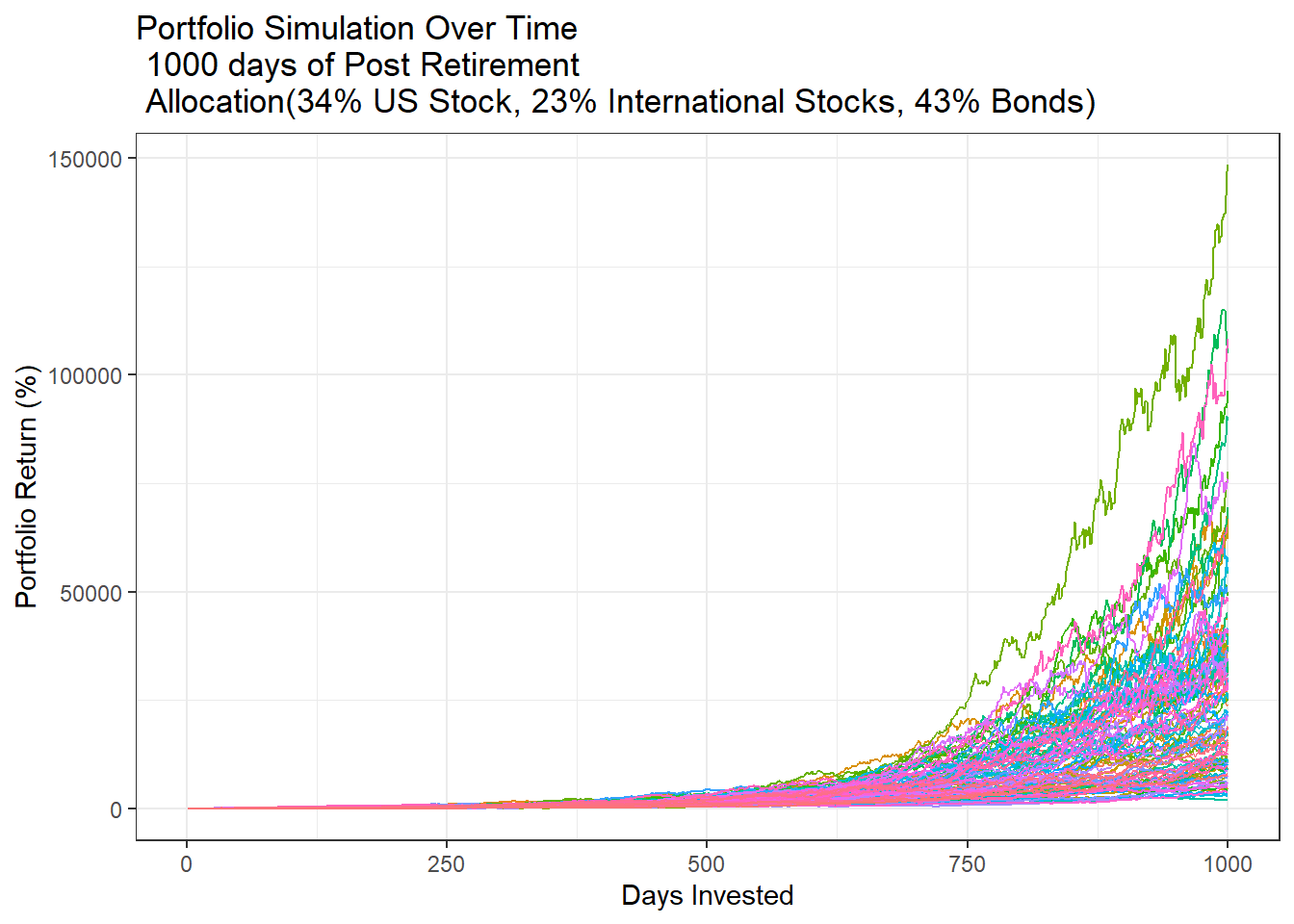
MONTE CARLO SIMULATION
Inspired from Youtube Video I tried doing Monte Carlo Simulation for the retirement portfolio returns for 1000 days
Warning in ((usequity.ret$US_equity_market_return/100) * 0.34) +
((int.ret$Int_equity_market_return/100) * : longer object length is not a
multiple of shorter object length
Code
monte_carlo_simulations<-function(return_vect,ndays=1000, n_sim=100){set.seed(0)return_vect=1+return_vectpaths<-replicate(n_sim, expr=round(sample(return_vect,ndays,replace=TRUE),2))#to seee if there are any tail eventspaths<-apply(paths,2,cumprod)paths<-data.table::data.table(paths)paths$days<-1:nrow(paths)paths<-data.table::melt(paths,id.vars="days")return(paths)}visualize_simulations=function(path){ggplot(path, aes(x =days, y =(value-1)*100, col =variable))+geom_line()+theme_bw()+theme(legend.position ="none")+labs( title ="Portfolio Simulation Over Time \n 1000 days of Post Retirement\n Allocation(34% US Stock, 23% International Stocks, 43% Bonds)", x ="Days Invested", y ="Portfolio Return (%)")}path=monte_carlo_simulations( return_vect=weighted.ret)visualize_simulations(path)
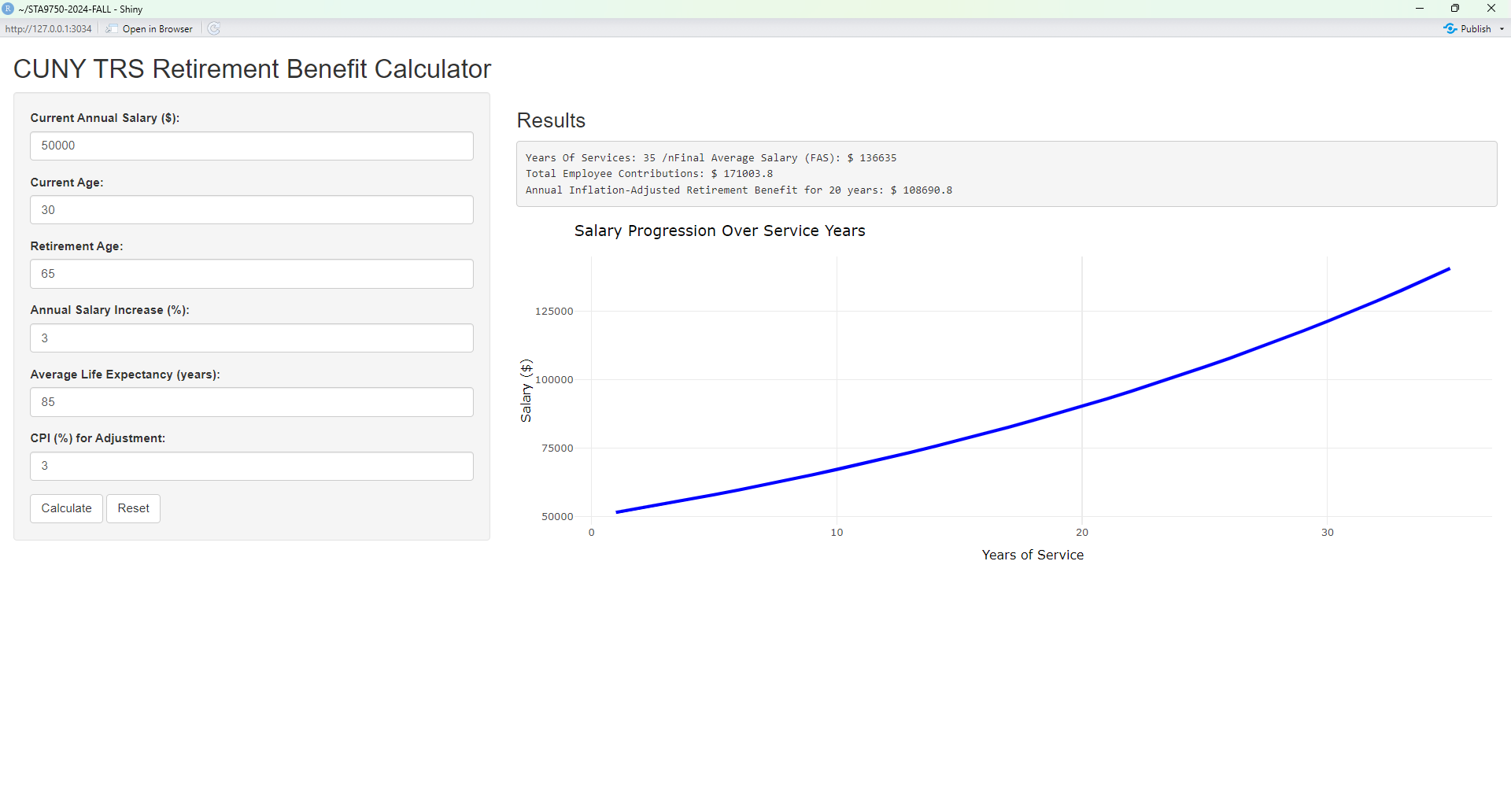
EXTRA CREDIT
I tried to create a shiny app for CUNY TRS Retirement Benefit Calculation. Unfortunately, I couldn’t publish it, below are the screenshot and codes for the CUNY TRS Retirement Benefit Calculator. Feel Free to replicate
Code
#|warning: false#|message: false#| echo: false# Load the shiny librarylibrary(shiny)
Attaching package: 'shiny'
The following object is masked from 'package:jsonlite':

    validate
Code
# Define the UIui<-fluidPage(titlePanel("CUNY TRS Retirement Benefit Calculator"),sidebarLayout(sidebarPanel(numericInput("salary", "Current Annual Salary ($):", value =50000, min =0),numericInput("age", "Current Age:", value =30, min =18, max =70),numericInput("retirement_age", "Retirement Age:", value =65, min =50, max =80),numericInput("annual_increase", "Annual Salary Increase (%):", value =3, min =0, max =20),numericInput("average_life_expectancy", "Average Life Expectancy (years):", value =85, min =70, max =100),numericInput("cpi", "CPI (%) for Adjustment:", value =3, min =0, max =10),actionButton("calculate", "Calculate"),actionButton("reset","Reset")),mainPanel(h3("Results"),verbatimTextOutput("results"),plotlyOutput("salary_plot"))))# Define the server logicserver<-function(input, output){output$results<-renderPrint({input$calculate# Trigger calculation when button is clickedsalary<-input$salaryage<-input$ageretirement_age<-input$retirement_ageannual_increase<-input$annual_increaseaverage_life_expectancy<-input$average_life_expectancycpi<-input$cpi/100# Convert to decimaltotal_contributions<-0years_of_service<-retirement_age-agelast_3_salaries<-numeric(3)retirement_benefit_years<-average_life_expectancy-retirement_age# Calculate salary progression over years of service based on the annual wage growthsalary_progression<-data.frame(year =(age+1):(retirement_age), salary =numeric(years_of_service))salary_progression$salary[1]<-salary# Define the employee contribution functionemployee_contribution<-function(salary){emp_rate<-ifelse(salary<=45000, 0.03, ifelse(salary<=55000, 0.035,ifelse(salary<=75000, 0.045,ifelse(salary<=100000, 0.0575, 0.06))))biweekly_contribution<-salary*emp_rate/26return(biweekly_contribution)}# Loop to calculate total contributions and final average salary (FAS)for(iin1:years_of_service){salary<-salary+salary*annual_increase/100biweekly_contributions<-employee_contribution(salary)# Update the last 3 years of salaryif(i>years_of_service-3){last_3_salaries[i-(years_of_service-3)]<-salary}total_contributions<-total_contributions+biweekly_contributions*26}# Compute the final average salary (FAS)FAS<-mean(last_3_salaries)# Define the annual retirement benefit functionannual_retirement_benefit<-function(FAS, years_of_service, retirement_benefit_years){if(years_of_service<=20){benefit<-0.0167*FAS*years_of_service}elseif(years_of_service==20){benefit<-0.0175*FAS*years_of_service}else{benefit<-(0.35+0.02*(years_of_service-20))*FAS}# Apply CPI adjustmentcpi_adjustment<-max(min(0.01+0.005*cpi, 0.03), 0.01)adjusted_benefit<-benefit*(1+cpi_adjustment)^retirement_benefit_yearsreturn(adjusted_benefit)}# Calculate annual retirement benefitadjusted_benefit<-annual_retirement_benefit(FAS, years_of_service, retirement_benefit_years)# Print the resultscat("Years Of Services:",years_of_service,"/n")cat("Final Average Salary (FAS): $", round(FAS, 2), "\n")cat("Total Employee Contributions: $", round(total_contributions, 2), "\n")cat("Annual Inflation-Adjusted Retirement Benefit for",retirement_benefit_years, "years: $", round(adjusted_benefit, 2), "\n")})output$salary_plot<-renderPlotly({salary<-input$salaryannual_increase<-input$annual_increaseyears_of_service<-input$retirement_age-input$age# Generate yearly salary datasalary_data<-data.frame( Year =seq(1, years_of_service), Salary =cumprod(rep(1+annual_increase/100, years_of_service))*salary)# Plot the salary progressionsalary_increase_graph<-ggplot(salary_data, aes(x =Year, y =Salary))+geom_line(color ="blue", size =1)+labs(title ="Salary Progression Over Service Years", x ="Years of Service", y ="Salary ($)")+theme_minimal()ggplotly(salary_increase_graph)})}# Run the applicationshinyApp(ui =ui, server =server)
Shiny applications not supported in static R Markdown documents